5.4. Colloid Postprocessing
5.4.1. Colloid output formats
Colloid output can be either in ASCII or raw binary format. A simple
example can be found at docs/tutorial/colloid-test1. Copy the
input file to a suitable location with name input and run the code:
$ ./Ludwig.exe
...
A single colloid configuration in ASCII format should be generated at
the end of this short run of 1000 time steps with name
config.cds00001000.001-001. The file can be inspected
with a suitable utility.
These files are used for the purposes of restarting the computation, but are not particularly convenient for visualisation. An extra post-processing step is typically required.
5.4.2. Visualising colloid positions
5.4.2.1. Generating a CSV file
One way to manipulate the colloid data to produce a format suitable for
visualisation is to use the extract_colloids utility found in the
util directory. This will reform the output file (either ASCII or
binary) to a comma-separated-values (CSV) file. In its most simple
form:
$ ./extract_colloids config.cds00001000.001-001
...
Wrote 10 colloids to colloids-00001000.csv
This CSV file holds (by default) the position and velocity of each particle.
5.4.2.2. Viewing the positions in isolation
The new CSV file can be read into, e.g., Paraview.
Open the
colloids-00001000.csvfile and read in using the CSV reader. (This will open a “spreadsheet” view in Paraview, which can be dismissed.)The first operation to perform is to add a
TableToPointsfilter (Filters->Alphabetical->TableToPointsfrom the pull-down menus).In the
Propertiessection ofTableToPointsset theX Columntoxfrom the pull-down menu, and likewise forYandZ. This associates the coordinates in the output data with the relevant columns in the CSV data.We will represent each colloid with a sphere. Add a
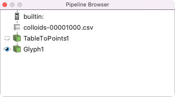
Glyphfilter to the output ofTableToPoints. In theGlyphproperties: forGlyph SourceselectSpherefrom the pull-down menu; forScaleselectNo scalae array; from theMaskingsection, selectAll pointsforGlyph mode.
This should provide a very simple picture of the relative positions of the colloids. The pipeline is set out below.
5.4.2.3. Adding lattice information
This simple picture does not contain any information about the size of the system, or the associated lattice quantities. This is most simply done by reading one of the associated lattice quantities produced at the same time (in this case the density and the velocity are available). This will automatically set the extents of the system in each co-ordinate direction.
One should then set the Scale factor in the Glyph properaties
to the appropriate colloid size (in this example, the radius is 2.3
lattice units).