5.3. Liquid Crystal Output¶

5.3.1. Liquid crystal order parameters¶

The dynamics of the liquid crystal problem are based on the symmetric, traceless, tensor order parameter \(Q_{\alpha\beta}(\mathbf{r};t)\). The model carries five independent components of this tensor in three dimensions, which are always stored to file as \(Q_{xx}, Q_{xy}, Q_{xz}, Q_{yy}\) and \(Q_{yz}\) (five scalar entities).

For the purposes of analysis and visualisation, it is actually preferable to consider a different set of quantities which are: the (scalar) order parameter, the director, and the (scalar) bi-axial order parameter. Specifically, the scalar order parameter is the largest eigenvalue of Q, the director is the associated eigenvector, while the bi-axial order parameter is related to the two largest eigenvalues. Physically, the scalar order parameter is expected to vanish at disclinations, and the director is the orientation of the rod-like molecules (a directionless vector); the bi-axial order parameter reflects the degree to which the order is ‘plate-like’ as against ‘rod-like’.

These latter quantities may be generated by diagonalising the tensor \(Q_{\alpha\beta}(\mathbf{r};t)\) at each position and time step. For any given problem, it may be relevant to look at one or more of these quantities.

5.3.2. Examples: processing LC output¶

We assume a computation has produced a binary file q-000010000.001-001 for some appropriate input configuration, along with the associated meta data file. Computing and storing the diagonalised quantities currently involves running the post-processing utility util/extract. Some example are given below.

5.3.2.1. VTK output for the director¶

From the command line, run

$ ./extract -k -d q-000010000.001-001
...
Writing computed director with vtk: lcd-000010000.vtk
Complete processing for q-000010000.001-001

The output here is a single file prefixed lcd with the director field as a vector.

5.3.2.2. VTK output for the scalar order parameter¶

For the scalar order parameter, use the -s option:

$ ./extract -k -s q-000010000.001-001
...
Writing computed scalar order with vtk: lcs-000010000.vtk
Complete processing for q-000010000.001-001

The output is a VTK file prefixed lcs with the scalar order parameter.

5.3.2.3. VTK output for the bi-axial order parameter¶

If required, use the -x option:

$ ./extract -k -x q-000010000.001-001
...
Writing computed biaxial order with vtk: lcb-00000000.vtk
Complete processing for q-000000000.001-001

This prodcues a file with the lcb prefix, which is the scalar bi-axial order parameter.

It is possible to combine the -s, -d and -x options to get more than one output at one time, if required. These VTK files may be visualised in the usual way.

5.3.2.4. Raw output for all quantities¶

The following command can be used:

$ ./extract -a q-000010000.001-001
...
Writing computed scalar q etc: q-000000000
Complete processing for q-000000000.001-001

This generates a single ASCII file with five columns. The order is \(s, d_x, d_y, d_z, b\) with \(s\) the scalar order parameter and \(b\) the bi-axial order parameter; the director is \((d_x,d_y,d_z)\). Note there is no file extension. Use the -b option instead if raw binary format output is wanted; the results are in the same order.

5.3.3. Example: visualising the scalar order parameter¶

Copy the example input docs/tutorial/liquid-crystal to an appropriate location and run the run. The input specifies a relatively small system with free energy parameters which are appropriate for blue phase one (with a cubic symmetry). The run is a short one to allow the initial conditions to relax, and we expect to be able to visualise the disclination lines in the final structure.

Run the input through the code, e.g.,

$ export OMP_NUM_THREADS=4
$ mpirun -np 1 ./Ludwig.exe blue-phase-visual.inp

This should take around minute (the exact choice of parallel options is not important). A single unprocessed order paarameter file q-000010000.001-001 should be produced. Run the extract program to obtain the scalar order parameter:

$ ./extract -k -s q-000010000.001-001

The resulting VTK file can be read into, for example, Paraview in the usual way. Apply a Contour filter to the data. It should be seen that the scalar order parameter varies between about 0.06 and 0.37. In order to obtain a coherent picture of the disclination structure a value of around 0.22 may be required for the isosurface value. In theory, the scalar order should vanish at the disclinations, but in the discrete model, this is not the case.

An example of the output is given below with a single isosurface contour value of 0.22. It can be seen that the disclinations are resolved at the level of around 2-3 lattice sites (the system size is 16 cubed.). A two-dimensional camera view has been selected to more closely reflect the cubic symmetry.

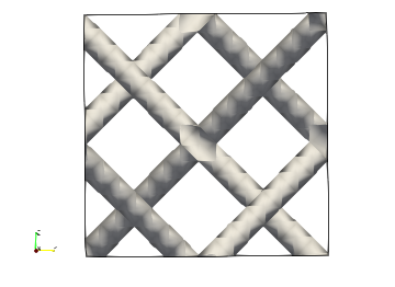
Disclination structure of blue phase one

If the contour value selected is too low, the picture will ultimately become fragmented and the isosurface discontinuous.

5.3.3.1. The director field¶

To view the director field in Paraview, proceed as for a vector field and apply a Glyph filter, but select Line instead of Arrow from the Glyph Type menu in the Glyph properties section. Some adjustment of the scale factor may also be required to obtain a reasonable picture.